AUTOMATED CURVE FITTING IN TABLECURVE 2D® : |
| |
TableCurve 2D Version 5 can fit multiple data sets automatically in a batch-processing mode. The data source is either an Excel spreadsheet (or multiple spreadsheets) or an instrument via a custom DLL. In addition to curve fitting, the Automation feature is available for other TableCurve features such as noise filtering, smoothing, local regression, splines and autoregressive modeling and prediction.
An example is the analysis of regional pulmonary ventilation of a 133Xe airway bolus using a scintillation camera. Since the bolus of xenon initially washes into the lung and subsequently washes out, we would expect one of the TableCurve intermediate kinetic functions to fit the data. See the TableCurve PDF nonlinear equation documentation for description of the intermediate functions. They represent measurement from the middle of three compartments. In our case the middle compartment is the lung with the airway and recirculation-via-organ-systems being the first and third compartments, respectively. Six of ten measured regions are shown in Figure 1. We want to fit all ten data sets as a batch and place the results in a Word file.
|
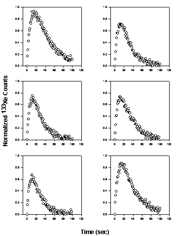
Figure 1.Regional pulmonary measurements of 133Xe washout.
|
Setting Up Automation
This is a two step procedure:
- select options to fit the first data set
- use these options for Automation to fit all data sets
Fit the First Data Set
You fit the first data set exactly the same way you normally use TableCurve except in this case we are going to restrict the fitting to the Kinetic equations. Open TableCurve and Import the file regional 133Xe washout.xls that you have downloaded. The Select Columns dialog, Figure 2, shows the data in columns A K of the Excel worksheet. This data is in X Many Y format with the X data in column A and the ten Y data sets in columns B - K.
|
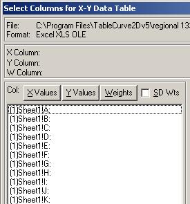
Figure 2. Select Columns dialog with time data in column A and ten regional scintillation measurements in columns B through K.
|
Select column A and B to be the X and Y data. At the Process menu select Edit Custom Equation Set. For each tab select Clear to deselect the equations except for the Kinetic tab - select all Kinetic equations. The dialog for the Kinetic tab is shown in Figure 3.
|
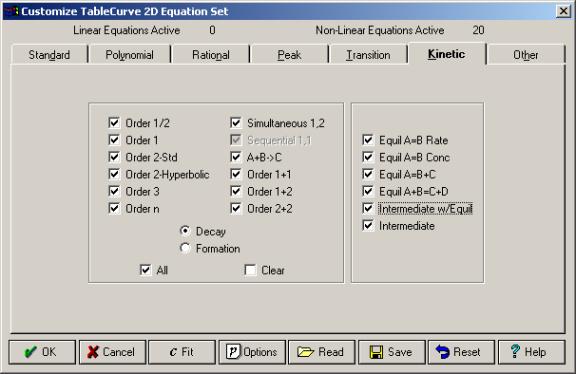
Figure 3. Kinetic tab of the Custom Equations dialog. All functions are selected. All functions in all other tabs are deselected.
|
Click the Fit button shown in Figure 3 to fit these equations to the data in columns A and B of the Excel worksheet. Click Graph Start to view the Review Curve Fit window and equations. The equation list shows the highest ranked equation (by either R2 or F-Statistic) is "Intermed11 c < d(a,b,c,d)" which is what we expected. For this data set the Equil111 equations are probably not significantly different from the Intermed11 equations.
|
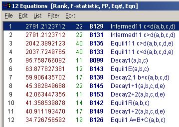
Figure 4. Equation list ranked by the F-statistic. The Intermed11 equations fit best.
|
Use Automation to Fit All Data Sets
We will now use Automation to fit all ten data sets with the equation selected to be the best during the fit of the first data set (Intermed11 c < d(a,b,c,d)) and place the results in a Word document. The Automation icon  is located at the bottom of the icon collection of the Review Curve-Fit window. Click on it to obtain the Automation dialog. is located at the bottom of the icon collection of the Review Curve-Fit window. Click on it to obtain the Automation dialog.
|
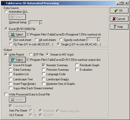
Figure 5. The Automation dialog. The data source is the Excel file ‘regional 133Xe washout.xls’. The Word output file is ‘133Xe washout output.doc’. Two output options, Curve-Fit Graph and Numeric Summary, are selected to view the curve fit results and obtain numeric parameter values for the ten data sets.
|
Our data source is an Excel file and our data is located in the first worksheet Single X (XY in cols AB, AC, AD,…) format. These are the options selected in the Data Source group box in Figure 5.
Select the options in the Output group box in Figure 5 to put the ten data set curve fit results in the Word document ‘133Xe washout output.doc’.
Click OK to curve fit the ten data sets with the Intermed11 c < d(a,b,c,d) equation.
Results of the Automated Fit
Graphs for the fit to each data set and the numerical fit results are placed into the Word document. The results for the second data set are representative and are shown in Figure 6.
|
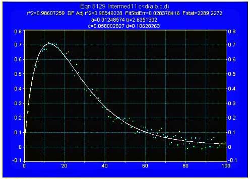
Figure 6. Automated results in the Word document for the second data set.
|
Rank 1 Eqn. 8129 Intermed11 c < d ( a,b,c,d)
|
| r2 Coef Det |
DF Adj r2 |
Fit Std Err |
F-value |
| 0.9860725867 |
0.9854922778 |
0.0283784161 |
2289.2272163 |
|
|
| Parm |
Value |
Std Error |
t-value |
95% |
Confidence Limits |
P>|t| |
| a. |
0.012485740 |
0.009232193 |
1.352413322 |
-0.00583761 |
0.030809087 |
0.17939 |
| b. |
2.635130203 |
0.450727827 |
5.846389021 |
1.740560240 |
3.529700167 |
0.00000 |
| c. |
0.058002827 |
0.007593421 |
7.638563579 |
0.042931989 |
0.073073665 |
0.00000 |
| d. |
0.106282625 |
0.014492888 |
7.333433025 |
0.077518254 |
0.135046997 |
0.00000 |
|
|
| Date |
Time |
| Feb 21, 2001 |
11:48:16 AM |
|
|
An excellent fit is obtained with and F ratio > 2000. Of physiological interest, the clearance constant (c parameter) is 0.058 sec-1. For all data sets this clearance rate ranges from 0.028 to 0.065 sec-1 with corresponding time constants of 35 (apical lung region) to 15 seconds (basal lung region).
Processing TableCurve Results
The Word file is an excellent report format but if you want to continue to process the results of TableCurve Automation then use the Excel output option.
|
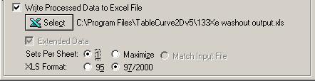
Figure 7. Options to place TableCurve Automation results into an Excel file.
|
The options shown in Figure 7 will place the fit results of the ten data sets into ten worksheets in the Excel file “133Xe washout output.xls”. You can then write a simple VBA macro in Excel to process these results. For example, you might create a table of lung clearance constant (c parameter) results for the ten data sets as a function of distance from lung apex to base. |